Linear Regression

Introduction and Background

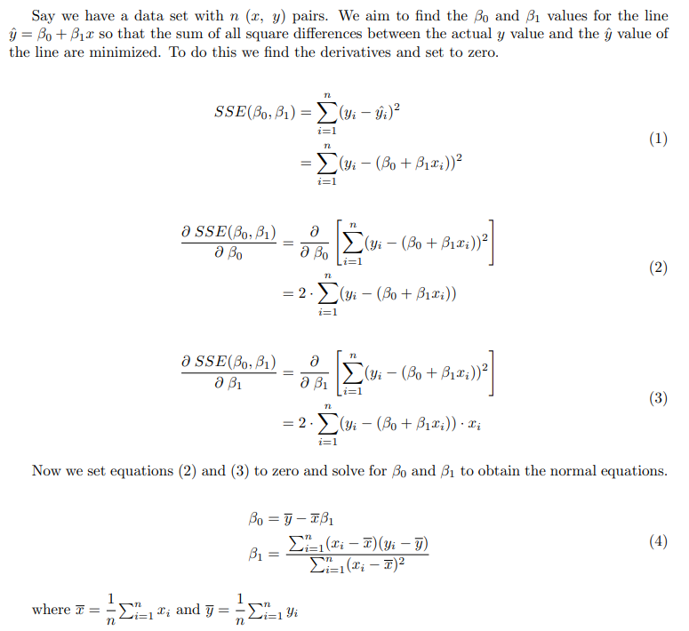
Linear regression is a method of approximating the relationship of as dataset with a line. The goal is to find a line of the form

that best explains our dataset. This is done by minimizing the sum of square errors of the line and the dataset. A quick derivation can be seen below.

Examples

- Creating a Dataset

The first thing you will need is a dataset that will be used to compute the line for the linear regression model. We create two arrays, x and y, which will be the features and targets respectively for the linear regression model. These arrays can hold any data you want but for this example we will stick with just a few simple numbers.

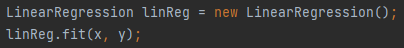
- Defining and Fitting the Model

We can now define our model by creating a LinearRegression object. In this example we name the linear regression model "linReg" but you can name it anything you want. Once the model has been defined we can "fit" the model to our dataset. This is the step that actually computes the line and finds the optimal parameters using the normal equations.

- Inspecting the Fit Model

If you want to view the details of the model, including the computed parameters of the line, you can call model_name.inspect(). Below you can see the code for this and the resulting output.

Making Predictions

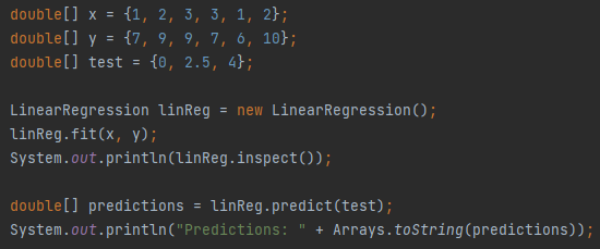
Now that the linear regression model has been fit, we can feed in new data and see what the model predicts the output to be. First, lets define a new array called test that contains the data we want to make predictions on.